Updated May 7, 2020 for the latest data and corrected an arithmetic error, which leads to revised conclusions.
Summary
The effective reproduction number is the number of people on average that a person will infect with a contagious disease. Through measures such as social distancing, we can reduce that number below a critical threshold of 1, at which point, if it stays there, the disease will hopefully die out without a cure or vaccine. This analysis has found that as of May 6, the effective reproduction number is above 1 at 1.247 (95% confidence interval = [1.235, 1.258]). It was trending strongly downward from mid-March to mid-April, however since mid-April it has levelled off, and is oscillating between about 0.86 and 1.36 at an average of 1.1 for the last 30 days. These results are updated from mid-April, and also correct an error which shows that the effective reproduction number is spending more time above 1 than previously shown, although it is still close to 1.
Although the disease is spreading fairly slowly as compared to its initial introduction in the U.S., social distancing and so forth as they have been implemented will not be sufficient to let the disease die out on its own. I am very skeptical of re-opening the economy, and will continue to be without far more robust contact tracing and testing systems in place, or a vaccine or cure. I also think the oscillations in the curves show that people are not observing social distancing as strictly on the weekends. Finally, I discuss the effect of undercounting on the calculation, and how it might be addressed.

The data for this analysis is available from the N.Y. Times. The code is here.
Introduction
In controlling the spread of an infectious disease, it is important to know how contagious it is. One simple way of quantifying is contagious is the number of people on average each infected person will directly infect. This is called the reproduction number, denoted 

One the reasons that 

The reproduction number is not constant over the course of an epidemic. It depends on anything that could affect how fast the disease spreads: the mechanism of transmission, how many people the average person interacts with, sanitation, etc. Controlling the disease means taking measures that get
Basic Reproduction Number
A disease’s basic reproduction number, denoted 
One estimate of COVID-19’s basic reproduction rate from the early phase of the first outbreak in China put
Effective Reproduction Number
So we can see why reducing the effective reproduction number, i.e., 


If we have a way of estimating 
The Renewal Equation
If we have data on the incidence of the disease, the rate at which new cases appear over time, and an estimate of its generation interval, the average amount of time it takes an infected person to directly infect one other person (the time to “generate” another case), we can estimate
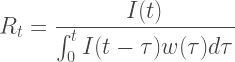


with


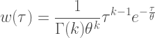
The COVID-19 mean generation interval 


Now let us see what the renewal equation is saying. It is just the number of new cases at time 
Discretization
The above form of the renewal equation, and the generation interval probability distribution are both in continuous form, as is the incidence function
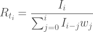
Where 


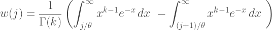
The two terms on the right side of the above equation are the upper incomplete gamma function evaluated at 

Our probability function with 

Estimation Method
To estimate 


Results
As of May 6, 2020, 

So initially we have some very high values for
First, let’s look at an 11-day moving average of

The 11-day average declines very slowly, then enters a steeper decline in mid-March (shortly after a national emergency was declared and social-distancing measures began). I’m going to guess that that slight decline before mid-March is probably due to a small but increasing subset of people following the news, anticipating the pandemic, and taking protective measures early on. If that’s true, then this makes the authorities, who failed to prevent what a significant number of average people could easily see coming, look very foolish.
The flat portion at the beginning of the curve suggests that the basic reproduction number is a bit less than 2.5. This is in good agreement with the estimate cited above of 2.24 (95% CI: 1.96, 2.55).
We also see that, since mid-April, the decline has pretty much levelled off, and on average, we have been hovering just above 1. The disease is current spreading but spreading slowly. The social distancing stopped the worst part of the crisis. However, it has not gotten us to a point where the disease will die out on its own without further measures.
Here’s what has been happening since the national emergency was declared on Mar. 13:

The beginning of the plot shows a spike occurring on March 19, followed by another pretty consistent decline until April 13. This spike is also apparent in the graph of the 11-day average. I am not sure why this spike appears. I will note that, consistent with a mean generation interval of 4.41 days, this is 4 days after the Center for Disease Control first publicly warned against gatherings of larger than 50 people on March 15. This is probably the point when many people and state and local authorities starting taking the need for social distancing much more seriously, because it became clear that most public places could not remain open. So, after this spike, we accordingly find a steep, then more shallow decline in 
Zooming in on the last 30 days, we see that the reproduction number has been oscillating between 0.86 and 1.36, at an average of 1.1.

Again, the social distancing got the reproduction number pretty close to 1. But the disease is still present and waiting to spread as soon as any of these measures are relaxed. Without other measures in place, like robust systems of contact tracing and accurate testing, to properly identify and isolate those people with the virus, it will spread unchecked and quickly lead back to a crisis. Personally, I don’t see much evidence that this is where it needs to be at a national level, and I expect the numbers are going to get significantly worse again in 2-3 weeks. I welcome any information that would prove me wrong on this point.
Bounces?
Note that in the above graphs there are regular bounces every 6-8 days. That is, the curve seems to repeatedly reach a local minimum, then start climbing to a peak about 3-4 days later, then falls back to a local minimum after another 3-4 days.
But once distancing measures are in place, they tend not to be lifted or relaxed, so we might expect the curve to be smoother (although maybe not monotonic). This could of course just be due to noise, but if it were then we should not expect to see such narrow confidence bands, because the estimation method simulated Poisson-structured noise. So unless the uncertainty in the incidence was way larger than a Poisson distributed error (which could easily be a difference of several hundred in either direction by the last dates of the data set), that should not be the source of spikiness.
The only explanation for these regular bounces which have been sustained consistently since at least the mid-March is that people are not observing social distancing as strictly on the weekends. If that’s true it would demonstrate how readily the rate of spread can climb with even slight relaxation of mitigation measures.
Undercounting of Cases
Another question we might ask is, since we know that there are probably a huge number of unreported cases, how does undercounting affect this estimation? It could if testing capacity has significantly changed recently to the estimate, but otherwise probably not. Why?
Suppose we somehow magically knew how many cases had not been reported on every given day since the first reported case. We could then a define a function 


Now, if 

I would guess this is a reasonable assumption because at first, there is very little testing capacity, but as cases and deaths mount, health authorities will ramp up their testing as fast as is feasible. However, they cannot do this forever and probably reach a plateau in the testing capacity at some point. After this point, we will have 
If we did have some estimate of 

For example, we might estimate by fitting an exponential curve based on observed testing policies. We might choose an exponential curve of the form 

To estimate 

We might reasonably guess that on day 1, the initial reports undercount by a factor of, say, 100. Then suppose that 30% of cases are asymptomatic, 56% are mildly symptomatic, 10% are severe requiring hospitalization, and 4% are critical, requiring ICU or ventilator treatment, possibly resulting in death (as is suggested here). Let’s say by day 28, all people requiring hospitalization, 14%, will be tested, but no one else. Then 


I didn’t bother to do this myself because I chose those numbers to estimate undercounting arbitrarily. I am just suggesting a way in which one might deal with undercounting.
Someone asked me about high false negative rates. The effect is the same. It will not change the calculation if the false negative rate is basically constant. A false negative rate of p is equivalent to assuming that the test has a 0% false negative rate, but failing to test a proportion of people equal to p.
Sources
[1] Shi Zhao, et al., Preliminary estimation of the basic reproduction number of novel coronavirus (2019-nCoV) in China, from 2019 to 2020: A data-driven analysis in the early phase of the outbreak. Int’l J. 92 Infectious Diseases 214-217 (March 2020). https://doi.org/10.1016/j.ijid.2020.01.050.
[2] Coburn BJ; Wagner BG; Blower S (2009). “Modeling influenza epidemics and pandemics: insights into the future of swine flu (H1N1)”. BMC Medicine. 7. Article 30. doi:10.1186/1741-7015-7-30.
[3] Ireland’s Health Services. Health Care Worker Information (PDF).
[4] Freeman, Colin. “Magic formula that will determine whether Ebola is beaten”. The Telegraph. Telegraph.Co.Uk.
[5] Shim, Eunha, et al. Transmission potential and severity of COVID-19 in South Korea. International Journal of Infectious Diseases 93 (2020) 339–344. https://linkinghub.elsevier.com/retrieve/pii/S1201971220301508;
[6] Nishiura, H & Chowell, G. The Effective Reproduction Number as a Prelude to Statistical Estimation of Time-Dependent Epidemic Trends. Mathematical and Statistical Estimation Approaches in Epidemiology. 2009 : 103–121.; Shim, et al. (2020).
[7] Shim, et al. (2020).
[8] Shim, et al. (2020); Nishiura & Chowell, 2009.
[9] http://wiki.stat.ucla.edu/socr/index.php/AP_Statistics_Curriculum_2007_Gamma
[10] Shim et al., 2020.
[11] Nishiura & Chowell, 2009.
[12] Nishiura & Chowell, 2009.
[13] Nishiura & Chowell, 2009.
[14] Chakraborty, S., & Chakravarty, D. Discrete Gamma Distributions: Properties and Parameter Estimations. Communications in Statistics – Theory and Methods, 41(18), 3301–3324 (2012). doi:10.1080/03610926.2011.563014
